Wind Turbine Blade: Fluid–Structure Interaction Analysis
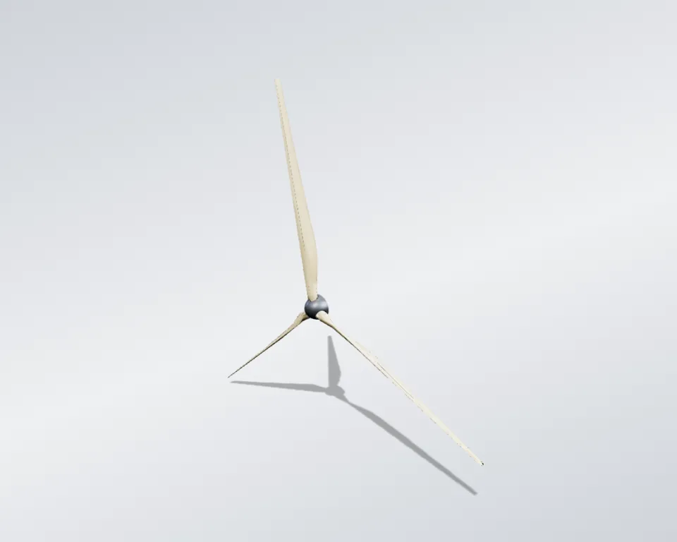
The goal was to see how a 41 m composite wind turbine blade bends under wind and rotation: its tip deflects 400.9 mm under the combined loads, and a hand check of the force at the blade root agrees within 0.1%. Lofted from 20 airfoil sections in SolidWorks, solved in ANSYS Fluent, then carried into ANSYS Mechanical (one-way fluid–structure interaction).
- Project
- Case study, Cornell University (online course)
- My role
- CAD, CFD, FEA and verification
- Tools
- SolidWorks, ANSYS Fluent, ANSYS Mechanical
- Method
- One-way fluid–structure interaction (CFD to FEA)
- 41.25maerodynamic blade span, from 20 airfoil sections
- 7.7Melements in the finest of 5 CFD meshes
- 400.9mmpeak tip deflection under combined loading
- ≤0.1%largest deviation of tip speed and root reaction force from hand calculations
Skills shown
How I did it
The study follows the same chain a blade design goes through before a structural sign-off: define the geometry and material system, resolve the aerodynamic loading, carry that loading onto a structural model, and check every step against an independent number rather than trusting the solver alone.
-
Model the blade
SolidWorks
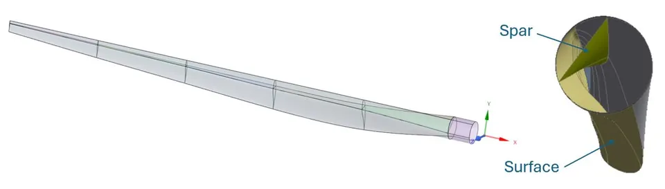
The blade is sized to the general class of a GE 1.5xLE-type 1.5 MW rotor: a 41.25 m aerodynamic span, lofted from 20 spanwise stations across three NREL airfoil families. Each airfoil section was sketched on its own spanwise plane, rotated about its leading edge to the local twist angle, and connected using an independent loft of the upper and lower surface curves, which keeps the leading- and trailing-edge feature lines unambiguous for the CFD and FEA meshers downstream.
The skin and spar are modeled as thin reference shells rather than solid bodies, split into five spanwise sections so the aerodynamic load can vary properly along the blade, and merged into one bonded multi-body part consistent with a co-cured composite structure.
- Aerodynamic span
- 41.25 m
- Twist, root to tip
- 42° → 0°
- Skin
- E-glass/epoxy laminate
- Spar
- Carbon-fiber/epoxy laminate
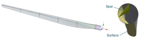
Skin and spar at the root cross-section. A single spar is placed at the quarter-chord, a common simplification in composite blade design. -
Simulate the airflow
ANSYS Fluent
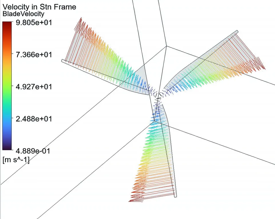
A single 120° periodic sector containing one blade was solved in a rotating reference frame at a rated-condition inflow (12 m/s, ω = 2.22 rad/s, tip-speed ratio ≈ 8), using the SST k-ω turbulence model: the standard choice for predicting boundary-layer separation on a lifting surface.
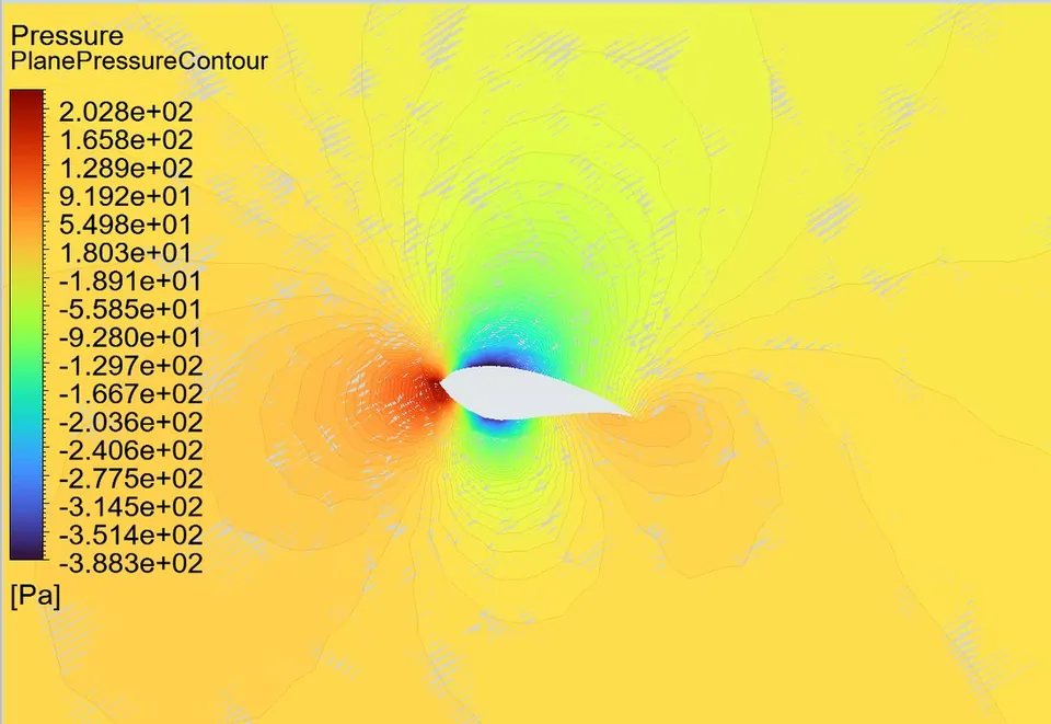
The pressure contour carries a clear asymmetry between the blade’s two surfaces. The deep blue region on the suction side reaches a substantially larger magnitude than the red and green regions, so that suction spike dominates the net pressure difference that generates lift.
- Inflow
- 12 m/s
- Angular velocity
- 2.22 rad/s
- Tip velocity
- ≈98 m/s
- Baseline mesh
- 356,628 elements
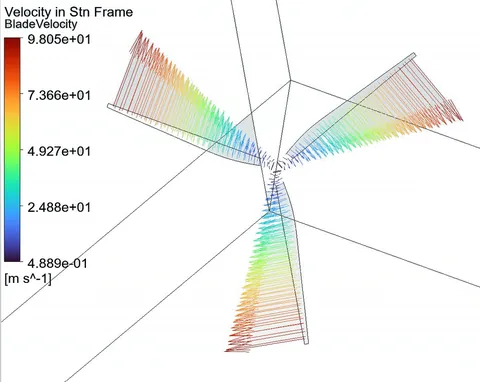
Blade-relative velocity, extrapolated to all three blades: velocity increases with radius, reaching ≈98 m/s near the tip. 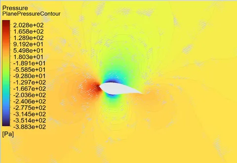
Static pressure around a representative cross-section: the suction peak that generates lift. 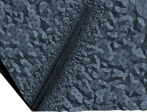
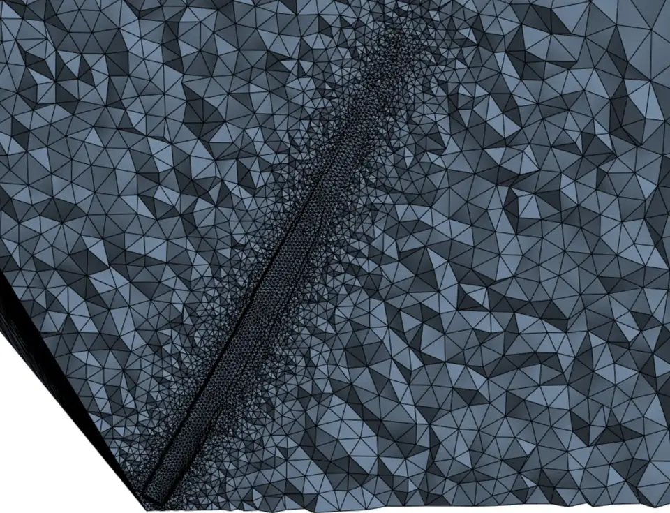
Boundary-layer inflation and near-field mesh refinement at the blade tip. -
Transfer the wind load
ANSYS Fluent to ANSYS Mechanical
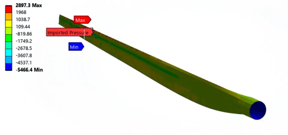
The converged CFD pressure field was mapped node-for-node onto an independently meshed shell-and-spar structural model, with 100% mapping fidelity (one-way FSI).
- Nodes mapped
- 100%
- Pressure range
- +2,897 to −5,466 Pa
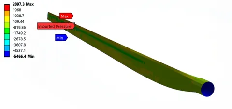
Aerodynamic pressure field imported from ANSYS Fluent onto the FEA shell mesh; 100% of target nodes received a mapped value. -
Calculate bending and stress
ANSYS Mechanical
The model was solved under combined aerodynamic pressure and centrifugal loading, with large-deflection stress stiffening enabled to capture how a spinning blade’s centrifugal tension increases its effective bending stiffness. A local coordinate system maps the orthotropic fiber direction onto the blade’s spanwise axis at every element.
- Tip deflection
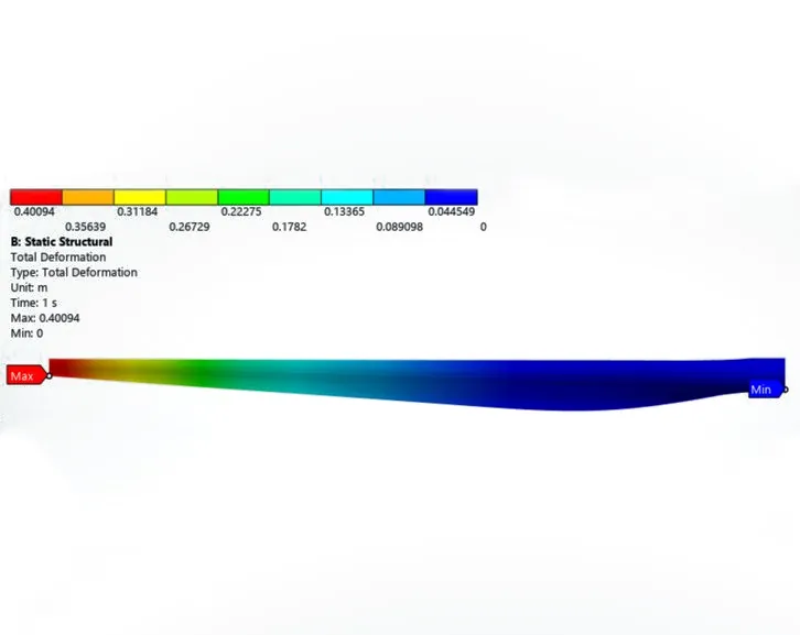
- 400.9 mm
- Peak stress
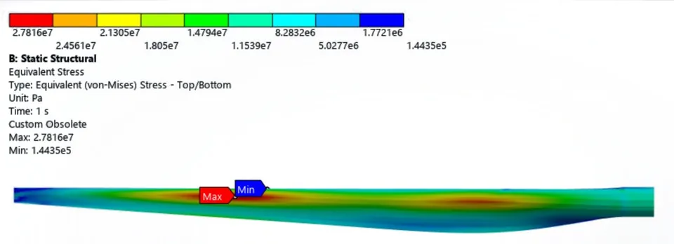
- 27.8 MPa
- Root reaction force
- 1,578.1 kN
- Shell elements
- 4,831
The structural load is taken from the 356,628-element baseline mesh, so the deformation and stress should be read as demonstrating a correctly executed FSI workflow rather than a fully mesh-converged design load. See the checks.
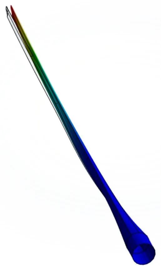
Deformation animation: the blade cycling from undeformed to its peak deflected shape under load. 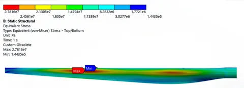
Equivalent (von Mises) stress: 27.8 MPa maximum, located at the outboard-root transition. Select to enlarge.
How I checked the results
Every headline result in this study is checked against an independent hand calculation, a mesh-sensitivity trend, or outside reference data rather than reported as a bare solver output.
≤0.1%
largest deviation of blade tip speed (CFD) and root reaction force (FEA) from independent hand calculations
Blade tip speed and root reaction force agree with independent hand calculations within 0.1%, and the CFD mass balance closes to about one part in a million of the throughput: strong confirmation that the boundary conditions, mass properties and load transfer are defined and applied consistently. The main open item is CFD mesh independence: the rotor power coefficient has not yet plateaued at the finest mesh tested (see the chart below), so it is carried forward explicitly rather than glossed over.
| Check | Result | Criterion | Status |
|---|---|---|---|
| CFD mass balance | −0.755 kg/s (≈0.0001% of throughput) | ≈ 0 | Pass |
| CFD residual convergence | All residuals ≤ 1×10⁻⁶ | ≤ 1×10⁻⁶ | Pass |
| Blade tip velocity (CFD vs. hand calc) | 98.05 vs. 98.12 m/s | Close agreement | Pass (0.07%) |
| Root reaction force (FEA vs. hand calc) | 1,578.1 vs. 1,576.3 kN | Close agreement | Pass (0.1%) |
| CFD → FEA load-transfer mapping | 100% of nodes mapped | 100% | Pass |
| Power coefficient vs. Betz limit | 13–42% (mesh-dependent) | < 59.3% | Pass, all meshes |
| Power coefficient vs. reference turbine | 41.5% (finest mesh) vs. 30% target | Order-of-magnitude agreement | Open, not mesh-converged |
| CFD mesh independence | Not reached at 7.7M elements | Plateau in Cp | Open |
Mesh refinement: power coefficient vs. mesh density
Rotor power coefficient (Cp) recomputed at five mesh densities. Hover a point for details.
The power coefficient nearly triples between the coarsest and finest mesh tested and has not yet leveled off at 7.7 million elements, though it stays well clear of the Betz limit throughout and brackets the 30% target computed independently from the real turbine’s rated performance.
The structural load in step 4 is taken from the 356,628-element baseline mesh, so the deformation and stress that follow should be read as demonstrating a correctly executed FSI workflow rather than a fully mesh-converged design load; closing that gap is the top follow-on item in the recommendations below.
Engineering judgment and recommendations
Beyond the pass/fail checks, the study points to where the model is solid and where it still needs work before it could support a production decision.
-
Flagged
Close out the CFD mesh dependency
The rotor power coefficient nearly triples between the coarsest and finest mesh tested (13.4% → 41.5%) without clearly leveling off. Because the structural load is taken from the coarser baseline mesh, the reported deformation and stress demonstrate a correctly executed FSI workflow rather than a final, mesh-converged design load. Re-run the structural pass once the CFD reaches grid independence.
-
Stress stiffening matters for a spinning blade
Enabling Large Deflection captures how centrifugal tension raises the blade’s effective bending stiffness, the same mechanism that raises a spinning turbine or helicopter blade’s natural frequency above its stationary value. Leaving it off would understate stiffness and overstate deflection.
-
Structural margin is generous, but indicative only
An indicative factor of safety near 20, against a representative composite allowable, reflects the deliberately conservative shell thicknesses used here, which also inflate the blade’s centrifugal load. A production design needs a ply-by-ply laminate check and a fatigue evaluation before that margin means anything for certification.
-
Opportunity: a mass-optimized thickness schedule
The current linear taper gives a blade several times heavier than a production blade of this span would weigh. Because the centrifugal load scales directly with mass, a tapered, laminate-optimized thickness schedule would cut both mass and load together, a natural next iteration for this model.
Technical details
Full settings, material data and verification for engineers who want to go deeper.
CFD and FEA setup Equations, domain, mesh, turbulence model, boundary conditions, elements
Aerodynamic analysis (ANSYS Fluent)
A single 120° periodic sector containing one blade was solved in a rotating reference frame at a rated-condition inflow (12 m/s, ω = 2.22 rad/s, tip-speed ratio ≈ 8), using the SST k-ω turbulence model: the standard choice for predicting boundary-layer separation on a lifting surface.
∇·(ρvrvr) + ρ(2ω×vr + ω×ω×r) = −∇p + ∇·τr
- Domain: 120° periodic single-blade sector, roughly 3–5× the blade radius out radially and 6× the span axially.
- Mesh: unstructured tetrahedral, 5-layer wall inflation, 0.30 m blade-surface sizing, 356,628 elements at baseline.
- Turbulence: SST k-ω, production limiter enabled, automatic near-wall treatment.
- Solver: coupled pressure-velocity scheme, second-order upwind, residuals driven to 1×10⁻⁶.
- Boundary conditions: 12 m/s velocity inlet at 5% turbulence intensity, pressure outlet, no-slip blade wall, rotationally periodic sides.
The pressure contour also carries a clear asymmetry between the blade’s two surfaces. On the color scale, the red (high positive pressure) and green (moderately negative) regions are of roughly the same magnitude, but the deep blue region on the suction side reaches a substantially larger magnitude than either. Because that suction spike outweighs the positive pressure on the windward side, it dominates the net pressure difference that generates lift.
Structural analysis (ANSYS Mechanical)
The converged CFD pressure field was mapped node-for-node onto an independently meshed shell-and-spar structural model (100% mapping fidelity), then solved under combined aerodynamic pressure and centrifugal loading, with large-deflection stress stiffening enabled to capture how a spinning blade’s centrifugal tension increases its effective bending stiffness.
[K]{d} = {F}
- Elements: 6-DOF shell elements (SHELL181/281-type), 4,831 elements and 4,671 nodes.
- Root boundary condition: all root nodes rigidly coupled to a single remote point at the hub, returning all six reaction components rather than forces alone.
- Loading: imported CFD pressure field plus the centrifugal body force from a 2.22 rad/s angular velocity, with Large Deflection (stress stiffening) enabled.
- Material orientation: a local coordinate system maps the orthotropic fiber direction onto the blade’s spanwise axis at every element, a required step for a physically meaningful anisotropic result.
Composite material model Homogenized orthotropic properties used in the FE model
The outer skin is modeled as an E-glass/epoxy laminate and the internal spar as a carbon-fiber/epoxy laminate: the standard industry split of a cost-effective glass skin carrying the aerodynamic shape and shear, with carbon concentrated in the spar cap where its stiffness-to-weight advantage matters most for flapwise bending. Both are represented in the FE model by a single homogenized orthotropic material.
| Property | Value | Unit |
|---|---|---|
| Density | 1,550 | kg/m³ |
| Young’s modulus, X (spanwise / fiber) | 113.75 | GPa |
| Young’s modulus, Y (chordwise) | 7.583 | GPa |
| Young’s modulus, Z (through-thickness) | 7.583 | GPa |
| Poisson’s ratio, XY | 0.32 | — |
| Poisson’s ratio, YZ | 0.37 | — |
| Poisson’s ratio, XZ | 0.35 | — |
| Shear modulus, XY | 5.446 | GPa |
| Shear modulus, YZ / XZ | 2.964 | GPa |
Benchmarked against handbook data for E-glass and carbon/epoxy laminates, these homogenized properties fall within typical ranges, and the resulting spanwise-to-chordwise stiffness ratio (≈15:1) is consistent with a carbon-weighted, spar-dominated section.
Analysis detail Each verification check expanded: what it establishes and what it doesn’t prove
Section “How I checked the results” summarizes each verification check in one line. Here, each check is expanded individually: what it establishes, the governing comparison, and what it does and doesn’t prove.
V1. Solver-Level Convergence & Conservation
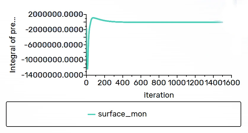
Confirms the discretized CFD equations were solved correctly, independent of whether the underlying model matches reality. Three physically distinct indicators are checked together rather than any one alone: global mass balance, scaled residuals, and the area-integrated blade-surface pressure, the quantity that actually determines the transferred structural load.
The net mass imbalance across domain boundaries is −0.755 kg/s against a throughput of over 660,000 kg/s; residuals for continuity, momentum, and turbulence transport all reach the target threshold; and the surface pressure monitor holds flat through the full 1,500-iteration run rather than merely meeting a residual threshold while the integrated load continued to drift.
V2. CFD Mesh Quality
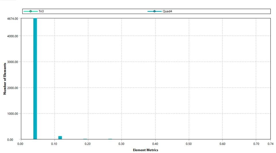
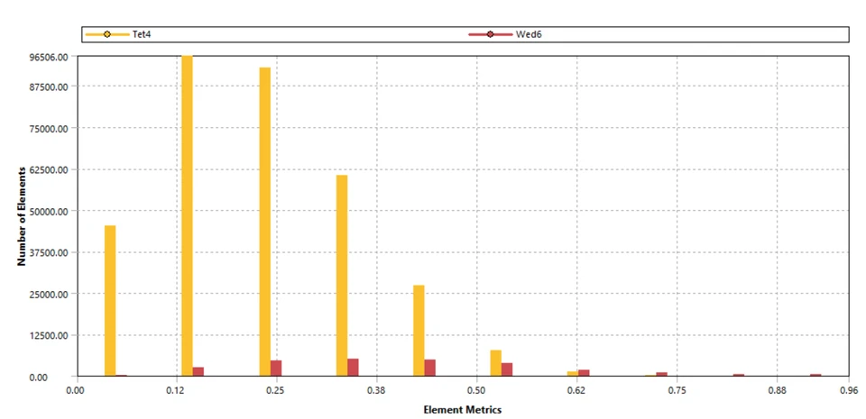
A converged solution is only meaningful if the underlying mesh is well-formed. Skewness is checked against the general-purpose quality bands published in the ANSYS Meshing User’s Guide, which is what a residual plot alone cannot confirm.
The great majority of the 356,628-element baseline mesh falls in the “excellent” (0–0.25) to “very good” (0.25–0.50) skewness bands, with no elements in the problematic ranges, a mesh well-suited to the SST k-ω solution without localized numerical-quality concerns that could otherwise corrupt the pressure and velocity gradients feeding the structural load transfer.
V3. Rotating-Frame Kinematics Cross-Check
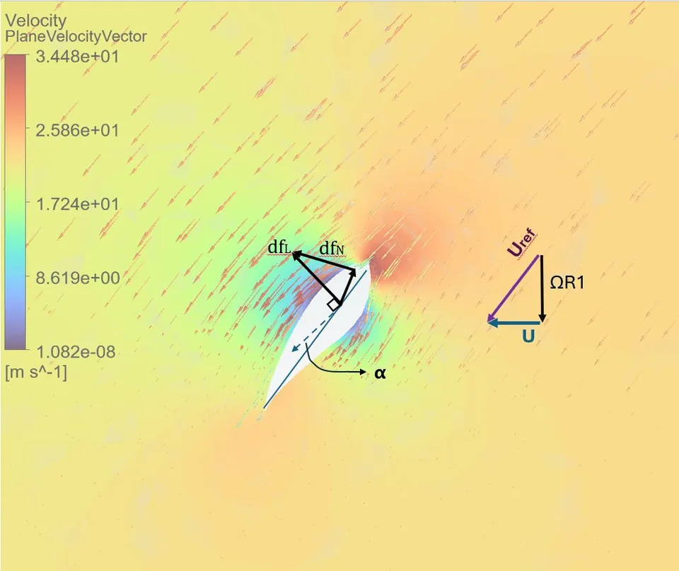
The rotating reference frame and angular-velocity boundary condition are checked against elementary rigid-body kinematics: for a point at radius r rotating at ω, tangential speed is v = rω, independent of anything the CFD solver itself computes.
vtip = rω = (44.2 m)(2.22 rad/s) = 98.12 m/s
The CFD-computed maximum blade-relative velocity matches the hand calculation to within 0.07%, a strong confirmation that the MRF rotational boundary condition (ω = −2.22 rad/s about +z) is correctly implemented. The velocity triangle shows the same relative-wind geometry that this check validates: axial inflow (U) and tangential blade speed (ΩR) combining into the relative wind that sets local angle of attack.
V4. CFD Domain-Size Adequacy
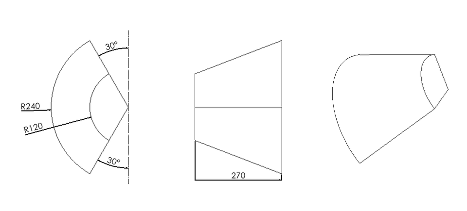
A formal domain-independence (blockage) study, re-solving on a larger domain and confirming the result is unchanged, was not run. In its place, the modeled clearance around the blade is checked qualitatively against general external-aerodynamics CFD guidance.
The domain extends radially to roughly 120–240 m (about 1.4–2.7 rotor diameters, with a 44.25 m tip radius) and axially to roughly 270 m (about 3 rotor diameters). That is well short of the 5–10 rotor diameters commonly recommended for external rotor aerodynamics, so blockage may inflate the computed loads and power coefficient somewhat. A dedicated domain-independence study remains open follow-on work.
V5. One-Way FSI Load-Transfer Fidelity
The converged CFD surface pressure must transfer completely and consistently onto the independently generated FEA shell mesh, with no un-mapped (extrapolated or defaulted) target nodes, for the two meshes to be considered geometrically consistent with each other.
ANSYS’s profile-preserving mapping reports 100% node-mapping fidelity: every target FEA node received a valid, interpolated pressure value from the source CFD mesh. The mapped range matches the suction-side low pressure and pressure-side higher pressure described qualitatively in the aerodynamic results, directly reflecting the net lift-generating pressure difference between the blade’s two surfaces. The imported field is shown in step 3.
V6. FEA Mesh Quality & Structural Reaction Cross-Check
As on the CFD side, the structural mesh is checked for skewness quality. Independently, the root reaction force is checked against a hand calculation for a point mass at fixed radius under centrifugal loading, a check that depends only on rigid-body kinematics, not on the FEA solver itself.
Fr = mrω² = (22,473 kg)(14.232 m)(2.22 rad/s)² = 1,576.3 kN
The 4,831-element FEA shell mesh shows no elements in the problematic skewness range. Independently, the ANSYS-computed root reaction force matches the hand calculation to within 0.1%, a strong confirmation that blade mass, center-of-mass location, angular velocity, and the remote-point root boundary condition are all correctly defined and consistently applied.