
Structural Health Monitoring: G. Meazza Stadium
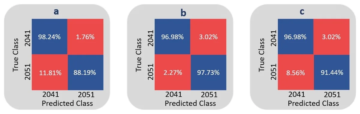
The goal was early warning of damage to the stands of Milan’s G. Meazza stadium: a classifier trained on two years of vibration data tells a healthy stand from a near-identical neighbor that represents the damaged state, with 97% accuracy on recordings it had never seen. Designed as the core of a real-time warning system, it misses 2.27% of the damage-proxy cases and raises 3.02% false alarms.
- Project
- M.Sc. thesis project
- Institution
- Politecnico di Milano
- Site
- Giuseppe Meazza Stadium, Milan
- My role
- Signal processing, feature selection, classifier design and validation
- Tools
- MATLAB (Signal Processing, Statistics & ML Toolboxes)
- 97%classification accuracy on 397 recordings the model never saw
- 2.27%missed-detection rate (damage read as healthy)
- 3.02%false-alarm rate (healthy read as damaged)
- 4,00010-minute recordings, mid-2018 to mid-2020
Skills shown
How I did it
Large structures age, get pushed past their original design life, and get used for loads they weren’t originally sized for, like concerts stacked on top of football matches. Manual inspection can’t keep pace with that. The goal was an automated, sensor-based system that flags a change in structural behavior as soon as it shows up in the vibration data, without needing a full analytical model of the structure.
- Detect a change in structural behavior automatically, from data the site already collects, without interrupting normal operation.
- Classify a reading as healthy or anomalous in real time, fast enough to be useful for a live monitoring system rather than a post-processed report.
- Avoid depending on a finite-element model of the whole structure, impractical to build and keep accurate for a structure that has been extended and modified multiple times since 1925.
- Validate the method against real, full-scale field data, not a lab specimen or a simulation.
- Reach a classification accuracy reliable enough to justify extending the method to the rest of the monitoring network.
-
The structure & monitoring network
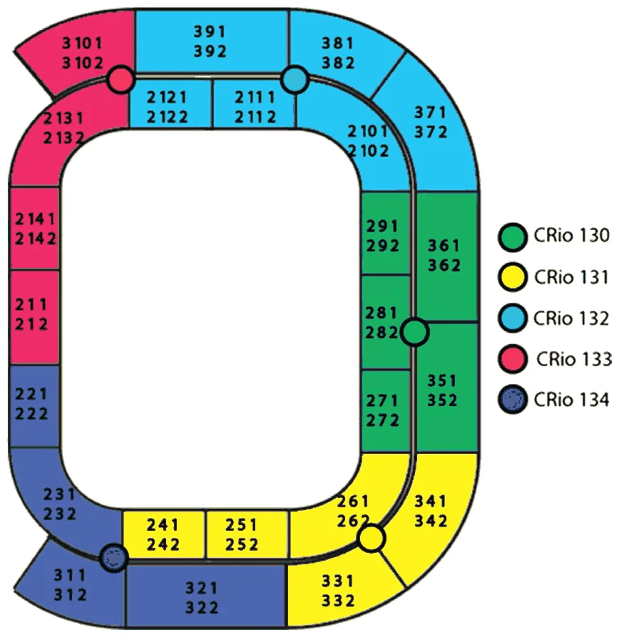
Permanent accelerometer network · 5 CompactRIO units
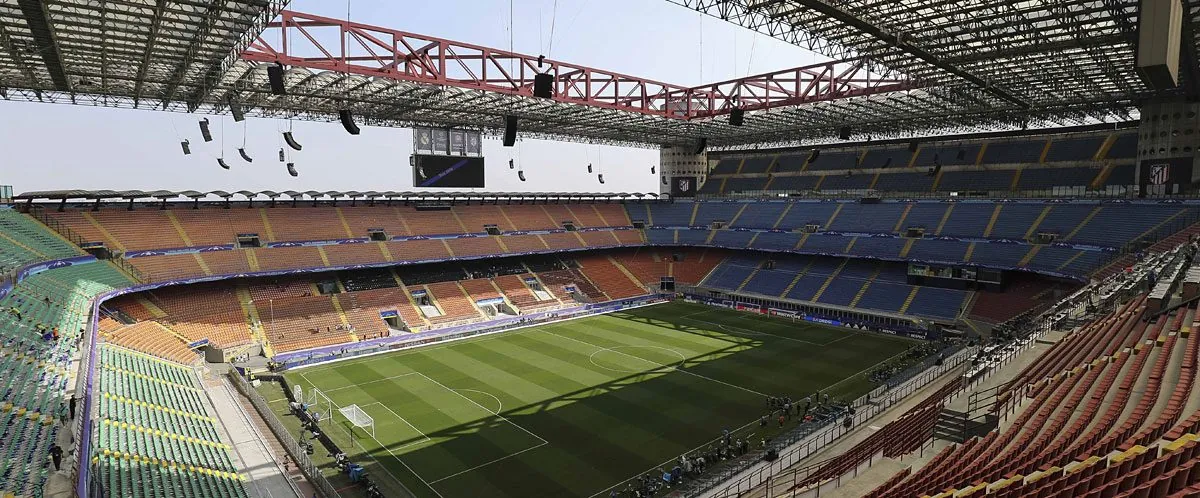
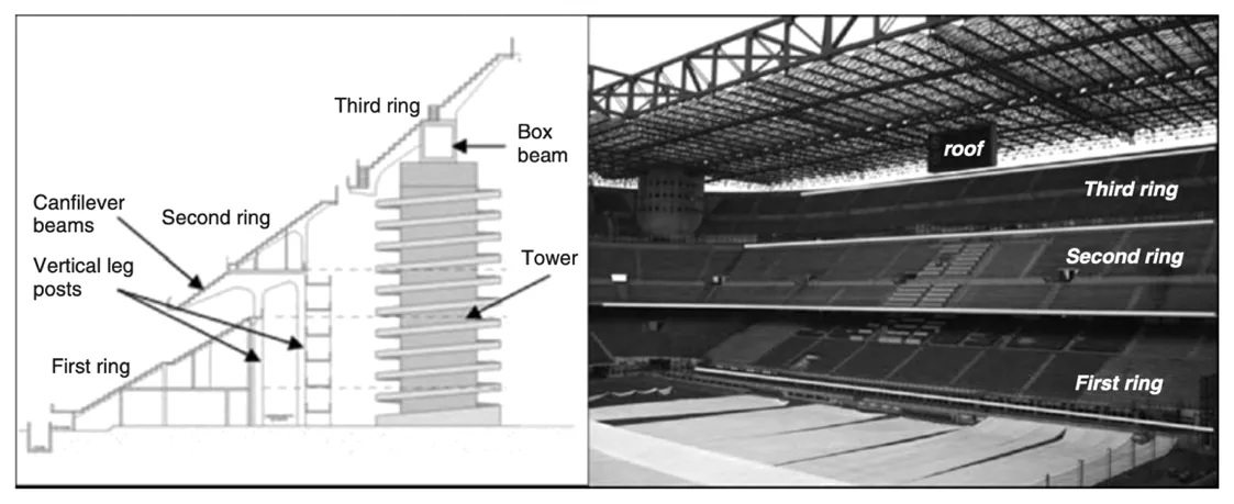
San Siro is Italy’s largest stadium and one of its structurally most complex: three seating rings, each built in a different era with a different structural system, plus an independently supported roof carrying its own load path.
- Seats
- 75,817, the largest stadium in Italy
- Structural rings
- 3, each a different era & system
- Accelerometers per monitored stand
- 2 (vertical + horizontal)
- Vibration data used
- 2018–20
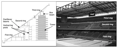
Cross-section and photo of the first, second, and third structural rings, each built in a different construction phase and load path. Select to enlarge. 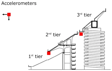
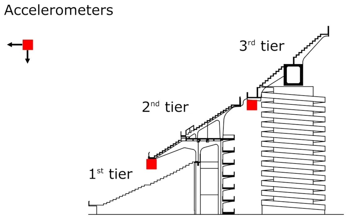
Accelerometer placement across the first, second, and third tiers. 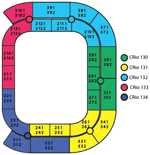
Layout of the permanent monitoring network: five National Instruments CompactRIO acquisition units, each covering a color-coded zone of stands. Select to enlarge. -
Method
MATLAB · vibration features + supervised classifier
Rather than model the whole structure, the approach compares new vibration readings against a known reference condition, conceptually the same thing as a modal analysis in FEA, where a shift in natural frequency or mode shape relative to a baseline model gets read as damage. Here, the baseline is a real, healthy stand instead of a healthy FE model.
Classification = Classifier (27 vibration-derived features, extracted from a 10-minute accelerometer recording)
- Two accelerometers (vertical + horizontal) per stand feed a permanent, wired monitoring network sampling at 128 Hz.
- Stand 2041 is treated as the healthy reference; a structurally similar neighboring stand, 2051, stands in for the damaged case. It is deliberately the hardest comparison available, since the two behave almost identically under normal loading.
- 27 features are extracted per recording: spectral features sensitive to changes in stiffness and mass, and statistical features sensitive to smaller changes the spectral ones miss.
- A classifier is trained on 70% of the dataset, validated on the remaining 30%, then stress-tested on recordings it never saw during training or tuning.
- Feature extraction, classifier training, optimization, and code generation for deployment were all done in MATLAB.
Anyone who has run a modal analysis in FEA has already done a version of this: perturb a model’s stiffness or mass, watch its natural frequencies and mode shapes shift, and read that shift as damage. This project runs the same logic on a real structure, with sensor data standing in for the FE model.
Same logic as an FEA modal damage check In an FEA modal study In this project Build the FE model of the healthy part or structure. Two real, near-identical stands stand in for the healthy and damaged model. Introduce a stiffness or mass change to represent damage. Accelerometers replace the FE solver as the source of dynamic data. Re-run the modal analysis. 27 features are extracted, several of them the same modal quantities an FEA report would list: dominant frequency, frequency ratio, spectral entropy. Compare natural frequencies and mode shapes to the baseline. A trained classifier replaces manual mode-shape comparison. A shift beyond tolerance flags damage. A deviation from the healthy baseline flags damage, in real time and on real data. -
Engineering process
Feature selection → classifier benchmark → tuning → blind test
Four stages, each narrowing in on a real-time, reliable classifier, plus one deliberate step back from the “best” validation result once it stopped generalizing.
Backing off from the best validation score to the best test score was a deliberate call: fewer iterations avoided overfitting to the training data, and generalized better to data the model had truly never seen. Because the blind-test results guided that choice, the 97% should be confirmed on a fresh hold-out set before deployment (see the recommendations).
- 1. Feature selection
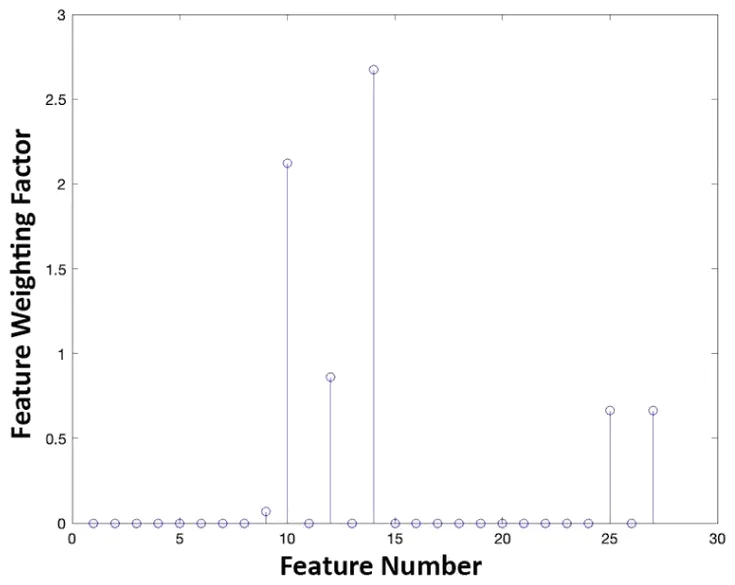
- All 27 features kept: 86.2% vs. 78.1% (5 NCA) and 80.2% (7 hybrid)
- 2. Classifier selection
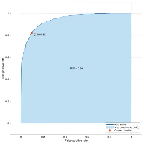
- Boosted Trees Ensemble, best of 30: 86.3%, AUC 0.94
- 3. Cost ratio & tuning
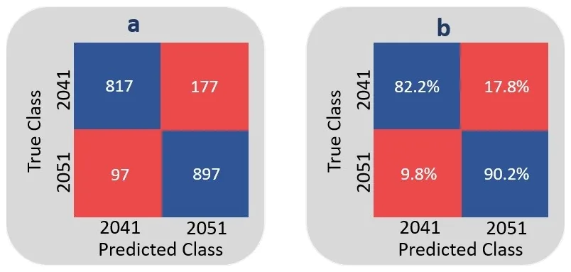
- 5 : 3 cost ratio; false alarms 17.8% → 12.6%
- 4. Independent blind test
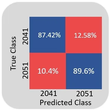
- 8 iterations, not 14: 2.27% / 3.02% errors
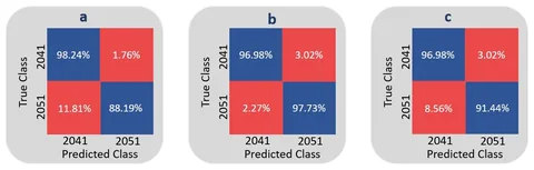
Blind-test confusion matrices at the 4th (a), 8th (b), and 14th (c) search iterations. 8 iterations gives the best, most balanced result. Select to enlarge. Each stage in full, with its figures, is in the technical details.
How I checked the results
The optimized classifier reaches 97% accuracy on data it never saw during training or tuning, with both error types low enough to trust for a real monitoring system.
97%
classification accuracy on the independent blind-test set (397 unseen recordings)
The model correctly separates the healthy stand from the damage-simulating stand in 97 of every 100 unseen recordings: a 2.27% missed-detection rate (damage-proxy stand read as healthy) and a 3.02% false-alarm rate (healthy read as damaged), achieved between two structurally near-identical stands, the hardest comparison in the dataset.
Classification accuracy through the engineering process
Validation / test accuracy at each stage, %. Hover a bar for details.
| Checkpoint | Metric | Result | Status |
|---|---|---|---|
| Feature-set selection | Validation accuracy, 27 features | 86.2% | Selected |
| Classifier benchmark | Best of 30 classifiers (Boosted Trees Ensemble) | 86.3% val., AUC 0.94 | Selected |
| Cost-ratio & hyperparameter tuning | False-alarm rate (healthy → damaged) | 17.8% → 12.6% | Improved, imbalance remained |
| Independent blind test (8 iterations) | Missed-detection / false-alarm rate | 2.27% / 3.02% | Validated |
| Overall result | Final classification accuracy, unseen data | 97% | Validated |
Engineering judgment and recommendations
Beyond the headline accuracy number, working through this pipeline surfaced a few things worth flagging before a method like this goes into a production monitoring system.
-
Flagged
No confirmed real-damage case yet
The damaged condition here is a proxy: a genuinely undamaged but structurally distinct stand standing in for stand 2041’s damaged state. The classifier has never been tested against a confirmed real damage event. Before relying on it operationally, it should be checked against retrofit, repair, or incident data as that becomes available.
-
Flagged
Confirm the 97% on a fresh hold-out set
The blind-test results also decided the final setting (8 search iterations instead of 14), so the same recordings served for both model selection and the final score. The 97% is therefore slightly optimistic; a new, untouched set of recordings, or a nested cross-validation, should confirm it before the classifier goes into service.
-
Opportunity: extend to farther, more different stands
Stands 2041 and 2051 were deliberately the hardest pair available, adjacent, near-identical, and easy to confuse. The same 27-feature pipeline should generalize more easily to stand pairs with more distinct dynamic behavior. Extending it there is the natural next step, with an even higher accuracy bar to clear.
-
Re-baseline after any structural modification
The healthy reference is empirical, drawn from stand 2041’s measured behavior between 2018 and 2020. Any future modification to that stand, or to the load path around it, would invalidate the baseline. The same discipline used to update an FE model after a design change applies here: re-collect reference data and retrain.
-
Cost ratio was tuned for this pair, not universally
The 5:3 cost ratio that balanced the error rates was found by trial and error on this specific stand pair. Rolling the same pipeline out to other locations should treat that ratio as a parameter to re-tune, not a constant to reuse, since baseline noise and structural similarity will differ from stand to stand.
Technical details
The data summary and each stage of the engineering process in full, for engineers who want to go deeper.
Data summary Instrumentation, recording and dataset: 128 Hz, 10-minute windows, 4,000 recordings, 70/30 split
Two years of field data, condensed into a dataset large enough to train a classifier and still hold back a genuinely independent test set.
| Parameter | Value |
|---|---|
| Instrumentation | |
| Sensors per monitored stand | 2 (vertical + horizontal accelerometer) |
| Acquisition hardware | 5× National Instruments CompactRIO units |
| Sampling frequency | 128 Hz |
| Recording | |
| Window length | 600 s (10 min), no overlap |
| Excitation condition | Ambient (empty stadium, no live event) |
| Collection span | Mid-2018 – Mid-2020 |
| Dataset | |
| Total recordings | 4,000 |
| Training / validation split | 70% / 30% |
| Independent blind-test set | ~397 recordings |
| Features extracted per recording | 27 (spectral + statistical) |
Engineering process: the four stages Feature selection, classifier benchmark, cost-ratio and hyperparameter tuning, independent blind test
Four stages, each narrowing in on a real-time, reliable classifier. The blind-test confusion matrices for the fourth stage are shown in step 3.
01. Feature selection: full set vs. reduced set
Approach
Fewer features generally means faster processing, so three feature sets were benchmarked head-to-head: all 27 features, 5 features selected by Neighborhood Component Analysis (NCA), and a 7-feature hybrid built by adding back two physically meaningful features.
Reducing the feature set cut processing time by up to 60%. However, since processing time remained real-time across all scenarios, this reduction came at too high an accuracy cost for a safety-relevant application. Therefore, all 27 features were retained for the remainder of the study.
02. Classifier selection: benchmarking 30 models
Approach
30 classifiers across eight families (decision trees, SVM, ensembles, neural networks, and more) were trained and validated on the same feature table to find the best fit for this data.
Ensemble methods and nonlinear SVM performed best; discriminant analysis failed outright, most likely because some features were constant or linearly dependent within a class, which makes the class covariance matrices singular. Processing time was fast enough across the board that accuracy, not speed, drove the choice.
03. Cost-ratio & hyperparameter optimization
Approach
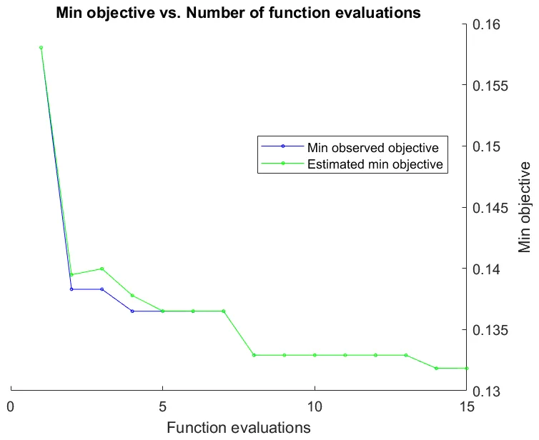
The raw classifier raised too many false alarms for a monitoring application (17.8% of healthy readings misread as damaged). Two levers were tuned to fix that: a misclassification cost ratio, biasing the classifier toward the healthy stand, and the classifier’s own hyperparameters, via Bayesian optimization.
Best cost ratio = 5 : 3 | hyperparameter search plateaued at 14 iterations
The trade-off improved the priority metric but didn’t fully resolve the imbalance, a sign that 14 iterations were starting to overfit. That is exactly what the next stage was designed to catch.
04. Independent blind test: guarding against overfitting
Approach
The 14-iteration model looked best on validation data, but validation data isn’t proof of real-world performance. The model was re-tested on ~397 recordings it had never seen, at three different hyperparameter-search lengths, to check which one actually generalized best.
Backing off from the best validation score to the best test score was a deliberate call: fewer iterations avoided overfitting to the training data, and generalized better to data the model had truly never seen. Because the blind-test results guided that choice, the 97% should be confirmed on a fresh hold-out set before deployment (see the recommendations).