
Carbon-Fiber Running Prosthesis
A carbon-fiber running blade for below-knee amputees must flex like a spring without breaking: under a 3000 N load it uses under half its allowed deflection and has an estimated 2.8× margin to failure. Composite shell FEA in Abaqus/CAE, checked against the physical bending-and-compression test it replicates; the spare margin leaves room for a thinner, springier blade.
- Project
- Case study, Politecnico di Milano
- My role
- Geometry, composite FEA and verification
- Tools
- Abaqus/CAE
- Method
- Composite shell FEA, Tsai–Hill failure criterion
- 18.8mmpeak vertical displacement, against a 40 mm allowable (47% of budget used)
- 0.355peak Tsai–Hill index away from the coupling singularity, against a failure threshold of 1.0
- ≈2.8×estimated load margin on the Tsai–Hill index
- 40plies, symmetric T300/5208 laminate, 8 mm thick
Skills shown
How I did it
Determine whether a curvilinear, 40-ply carbon-fiber blade survives its structural reference load with margin to spare, and confirm the model is solved correctly and represents the physical test it stands in for, before either result is used for a design decision.
- Predict displacement and ply-level Tsai–Hill failure index under a 3000 N axial reference load.
- Verify the model satisfies equilibrium and its own boundary conditions.
- Confirm the model replicates, feature for feature, the physical bend-and-compression test it stands in for.
-
Start from the physical test
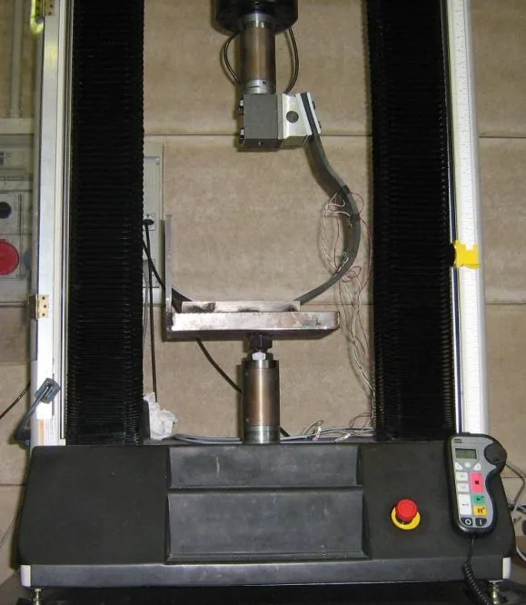
Test setup
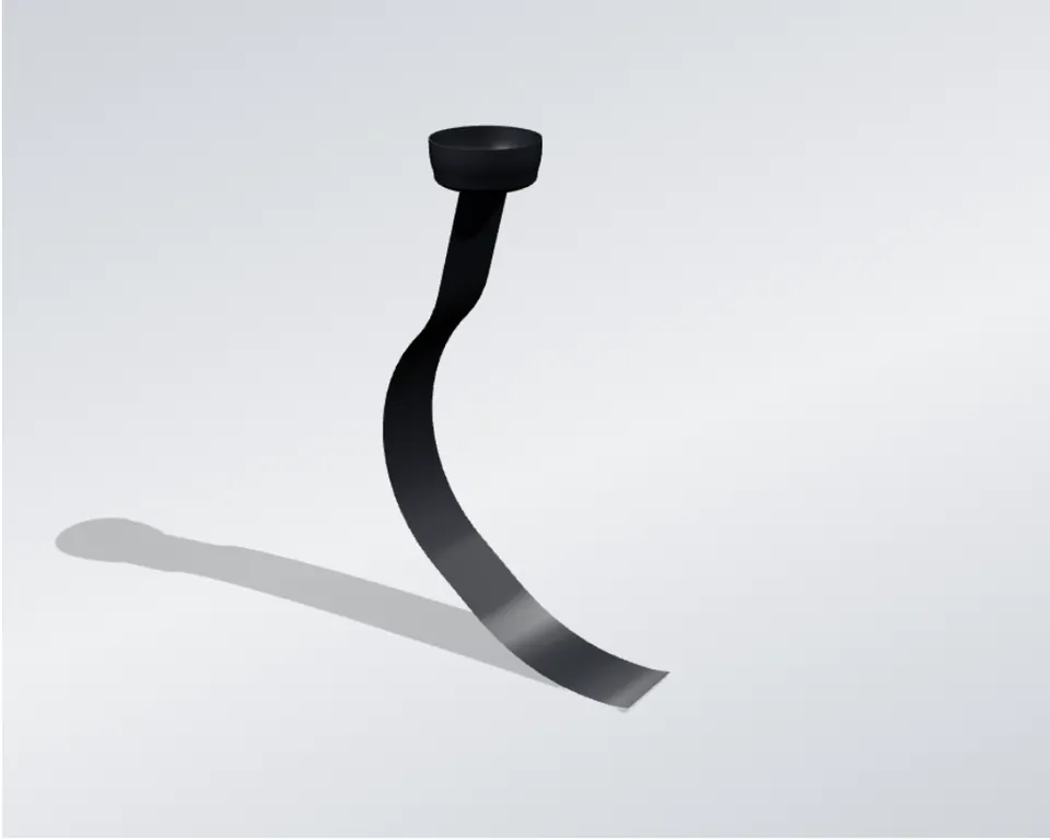
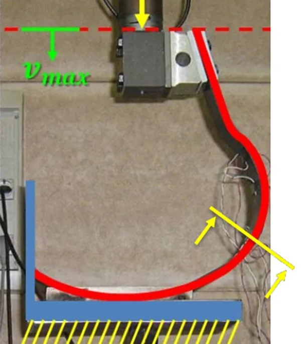
The prosthesis is a single curvilinear carbon-fiber blade that replaces both the foot and the distal shank. Every boundary condition in the model mirrors this physical bending-and-compression rig directly, rather than a generic idealization: the socket end couples to a reference point, the plantar end contacts two rigid plates through frictionless contact, and the 3000 N load and 40 mm allowable deflection carry over from the test’s own load and stiffness criteria.
- Axial reference test load
- 3000 N
- Laminate
- 40 plies, symmetric T300/5208, 8 mm
- Parts
- 2: deformable blade shell + rigid ground fixture
- Reference point
- 1, kinematically coupled at the socket
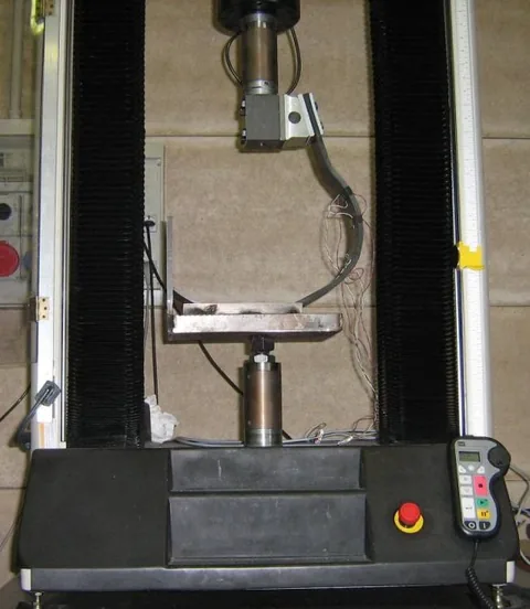
Bending-and-compression test rig, Structures Laboratory, Politecnico di Milano. 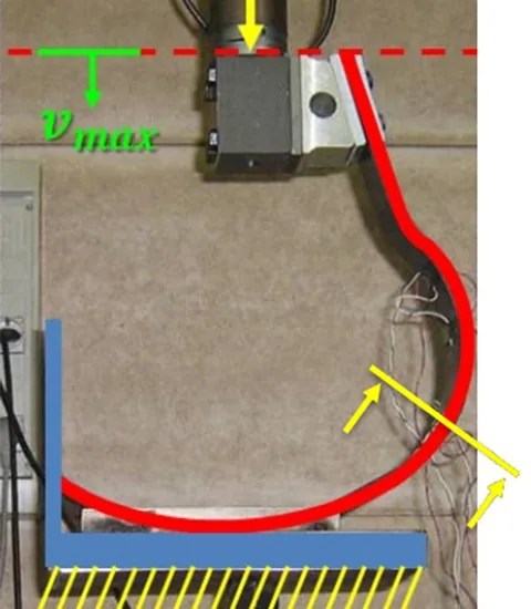
Same rig annotated with load direction, vmax, and the boundary conditions carried into the model. -
Define the geometry
Parametric profile
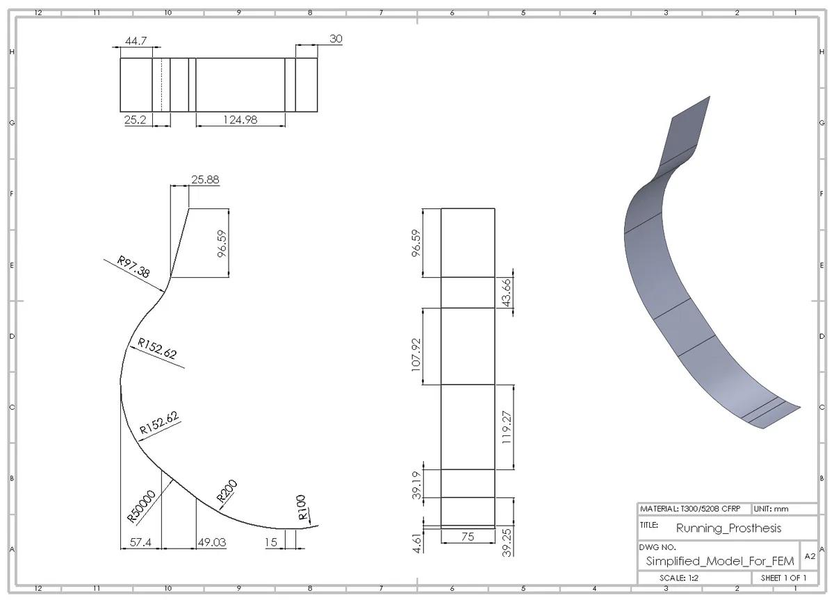
The free-form CAD blade is reduced, for this analysis, to a single dimensioned profile: a short tapered transition at the proximal (socket) end followed by a continuous run of tangent circular arcs that reproduce the blade’s C/J curvature down to the plantar tip. This parametric definition, not an imported free-form surface, is what was meshed and analyzed in Abaqus.
- Material callout
- T300/5208 CFRP
- Drawing scale
- 1:2, all dimensions in mm
- Primary bend radius
- R152.6 mm (two tangent arcs)
- Transition and tip arcs
- R97.4–R100
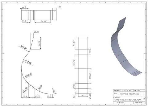
Simplified geometry used for the FE model: proximal taper, tangent-arc profile, cross-sectional stations, and the resulting 3D surface. Select to enlarge. -
Build the composite shell model
Abaqus/CAE
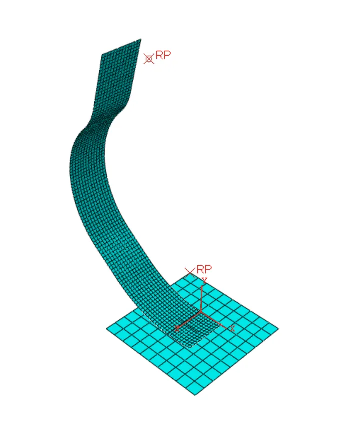
The assembly comprises a deformable composite shell (the blade) and a rigid fixture (the loading and ground-contact plates). The blade is meshed with quadratic, reduced-integration shell elements; the rigid fixture with a coarser linear mesh, since it carries no stress solution of its own.
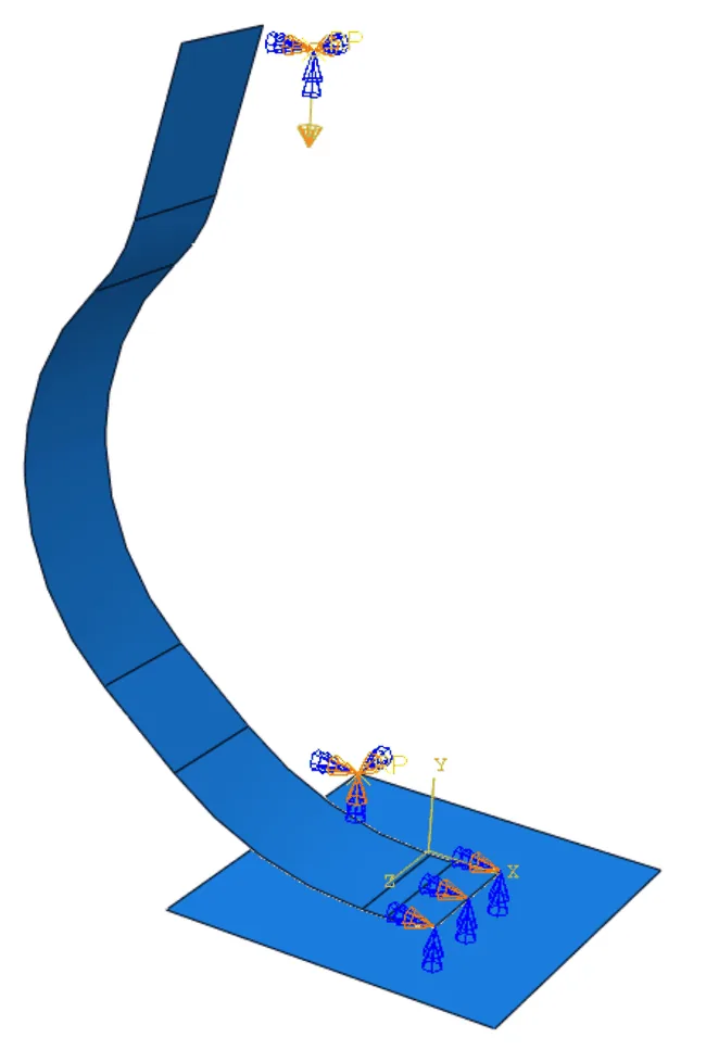
Every ply is unidirectional and oriented at 0° along the blade’s curvilinear axis, chosen to maximize axial stiffness since the dominant load path under the reference load runs along the blade’s length. The ply is defined as an orthotropic lamina from properties characterized in-house for this T300/5208 system (E1 = 131 GPa, longitudinal strength 1448 MPa). The strength is close to the widely used Tsai–Hahn reference value (1500 MPa), while the modulus is below its 181 GPa, which makes the deflection estimate conservative. Loads and restraints mirror the physical rig directly: the load point is free only along the load line, the ground fixture is fully fixed, and the blade’s plantar edge is restrained laterally while free to flex in-plane.
- Parts
- Composite blade shell + rigid ground fixture
- Plies modeled / physical
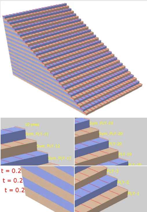
- 20 / 40 (symmetric, 8 mm total)
- Shell element size, blade
- 6 mm
- Element
- S8R5, 8-node quadratic shell, reduced integration
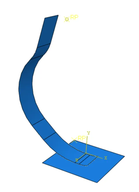
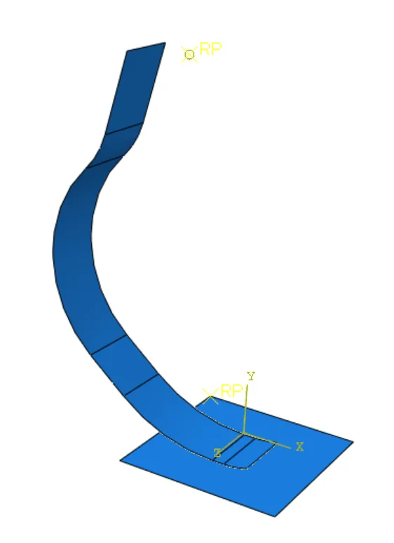
Assembly: blade shell + rigid ground fixture, with both reference points. 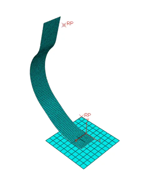
Mesh on the assembled model: quadratic shell elements on the blade, a coarser mesh on the rigid ground fixture. 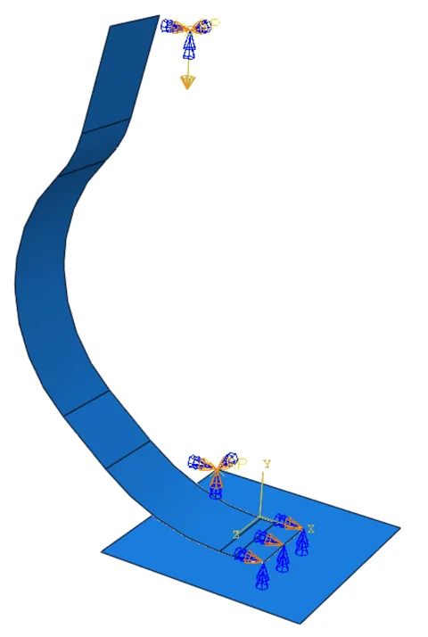
Boundary conditions and applied load on the assembled model. 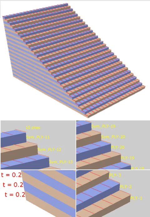
Ply stack-up: 20 modeled plies (PLY-1–20) mirrored by Abaqus into a symmetric 40-ply, 8 mm laminate, each ply 0.2 mm thick. -
Read the results
Abaqus/CAE
Both governing checks clear their limit with margin under the 3000 N reference load.
Displacement is probed directly at the loaded reference point: δmax = 18.8 mm (−18.805 mm at node 441), a smooth, monotonic deflection consistent with a curved cantilever compressed at its loaded end.
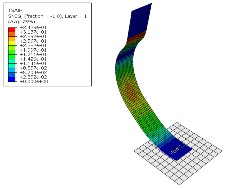
Tsai–Hill is evaluated ply by ply (Abaqus reports its square root as TSAIH, so TSAIH = 1 marks failure). The raw contour peaks, up to 0.448, sit directly at the idealized point-coupling constraint, an artifact of concentrating load through a single reference point rather than a real stress riser. Probing away from that region gives the representative peak of 0.355 used throughout this report, an estimated load margin of about 2.8×.
- Peak vertical displacement
- 18.8 mm (of 40 mm)
- Representative Tsai–Hill peak
- 0.355 (of 1.0)
- Raw peak at the coupling
- 0.448
- Estimated load margin
- ≈2.8×
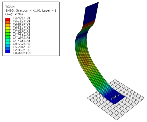
TSAIH contour, outer ply. The red patch at the top is the coupling-constraint artifact; the representative peak (0.355) is probed away from it. Select to enlarge.
How I checked the results
Before either result is used for a design decision, the model is checked two ways: has it been solved correctly, and does it represent the real prosthesis and test.
Structural margin against each limit
Percentage of the allowable limit used at the 3000 N reference load. Hover a bar for detail.
| Check | Result | Limit | Status |
|---|---|---|---|
| Peak vertical displacement | 18.8 mm | ≤ 40 mm | Satisfied |
| Peak Tsai–Hill index (away from singularity) | 0.355 | < 1.0 | Satisfied |
- Done: Reaction forces at both reference points balance the applied load, and the contact solution shows no interpenetration, both standard Abaqus diagnostics.
- Done: The peak Tsai–Hill value is probed away from the coupling singularity (0.355 vs. a raw 0.448) and decreases toward the laminate mid-plane, as expected for combined bending.
- Done: Boundary conditions replicate the physical test rig feature for feature (step 1), validated for setup fidelity.
- Outstanding: a quantitative strain-gauge/DIC comparison against the physical article, and a documented mesh-convergence study, before this model is relied on beyond a structural screening role.
An independent order-of-magnitude check, idealizing the blade as a curved composite cantilever using the ply’s own axial modulus, confirms the FE displacement is dimensionally consistent with the laminate’s stiffness. The blade’s width and curvature profile is now available in parametric form (step 2); completing the full closed-form comparison against it remains near-term follow-on work.
Engineering insights and recommendations
The structural check passes comfortably. The more interesting question is what that margin means for a component whose job is to store and return elastic energy, not just survive a proof load.
-
The 40-ply baseline is likely over-stiff for its job
The blade uses only 47% of its allowable deflection budget at the reference load. Since stored elastic energy scales with ½Fδ, that’s roughly 28 J stored against about 60 J the same envelope would allow at full deflection, close to twice the recoverable energy per stride for the same peak load. That margin reads as a design opportunity, not just a safety cushion.
-
Fatigue life is the next required check, not this one
This is a single static load case; a running prosthesis sees a ground-contact cycle on every stride, putting it deep into the high-cycle fatigue regime over a competitive career. A dedicated S–N or stiffness-degradation characterization is recommended before any thinner design is finalized.
Technical details
The material check behind the T300/5208 choice, for engineers who want to go deeper.
Material selection T300/5208 CFRP checked against E-glass/epoxy, Ti-6Al-4V and Al 7075-T6
Check the material
The original brief specified T300/5208 carbon-fiber epoxy without further justification. Because material choice governs stiffness, strength, energy return and cost at once, it’s checked here against three realistic alternatives before being adopted.
T300/5208 offers about four times the specific modulus of E-glass epoxy and over three times that of titanium or 7075 aluminum, so the blade reaches its stiffness at a fraction of the mass. More importantly for a device that works as an elastic spring, it can store several times more elastic energy per kilogram before failure than either metal, and carbon-fiber blades sit at the high end of the energy-return range reported for running prostheses (see the table). That combination, plus a peak Tsai–Hill index that stays well below 1 under the reference load, confirms the original material choice.
| Property | T300/5208 CFRP | E-glass/epoxy | Ti-6Al-4V | Al 7075-T6 |
|---|---|---|---|---|
| Density | 1.55 g/cm³ | 1.90 g/cm³ | 4.43 g/cm³ | 2.81 g/cm³ |
| Specific modulus (E1/ρ) | ∼85 | ∼21 | ∼26 | ∼26 |
| Long. tensile strength | 1448 MPa | ∼700–1000 MPa | ∼880 MPa | ∼503 MPa |
| Elastic energy return* | 63–95% (high end) | lower end of range | not used in RSPs | not used in RSPs |
*For complete running-specific prostheses of the stated material family, not a coupon-level property.