Turbulent Flow CFD Validation of a NACA 0012 Airfoil
The goal was to test whether a CFD simulation of airflow over a wing section can be trusted: lift matched NASA wind-tunnel data within 1–2%, and a 40% drag over-prediction most likely comes from one fixable meshing choice. Two-dimensional RANS simulation of turbulent flow over a NACA 0012 airfoil at a high Reynolds number.
- Project
- Case study, Cornell University (online course)
- My role
- Geometry, meshing, CFD and validation
- Tools
- ANSYS Meshing, ANSYS Fluent, CFD-Post
- Method
- 2D steady RANS, Realizable k-ε
- 1.059lift coefficient, ≈1–2% below the NASA reference
- +40%drag over-prediction, likely cause identified
- 6×10⁶chord-based Reynolds number, at 10° angle of attack
- 3/4validation & verification checks satisfied
Skills shown
How I did it
Check whether a steady RANS CFD methodology, built up from first principles and applied to a well documented benchmark airfoil, predicts lift and drag accurately enough to trust on a new, less characterized geometry.
-
Set up the case
ANSYS Meshing
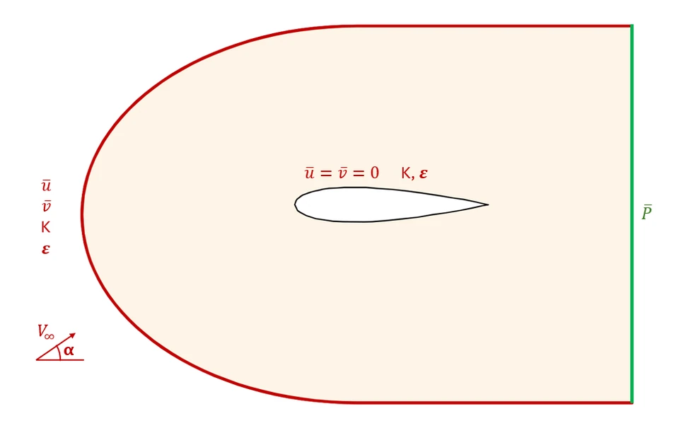
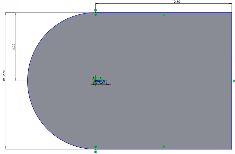
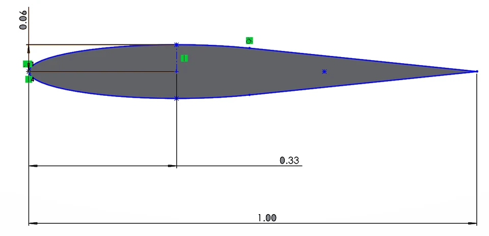
A single 2D symmetric airfoil section in a large far field domain, set up to isolate one steady operating point before any mesh or turbulence model refinement is attempted. The NACA 0012 profile has a 1.0 m chord, and the domain is sized to 12.5 chord lengths from the airfoil in every direction, with free stream velocity and turbulence quantities at the far field inlet, static pressure at the outlet, and the no-slip condition at the airfoil surface.
- Reynolds number
- 6×10⁶
- Angle of attack
- 10°
- Chord
- 1.0 m
- Domain extent
- 12.5 chords
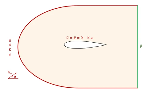
Boundary conditions applied to the domain: free stream velocity and turbulence quantities at the far field inlet, static pressure at the outlet, and the no-slip condition at the airfoil surface. 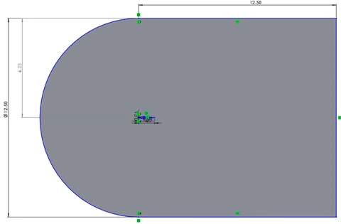
Far field domain sketch, sized to 12.5 chord lengths from the airfoil in every direction. 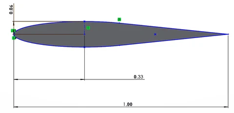
Dimensioned NACA 0012 profile used to build the flow domain, chord length 1.0 m. -
Build the mesh
ANSYS Meshing
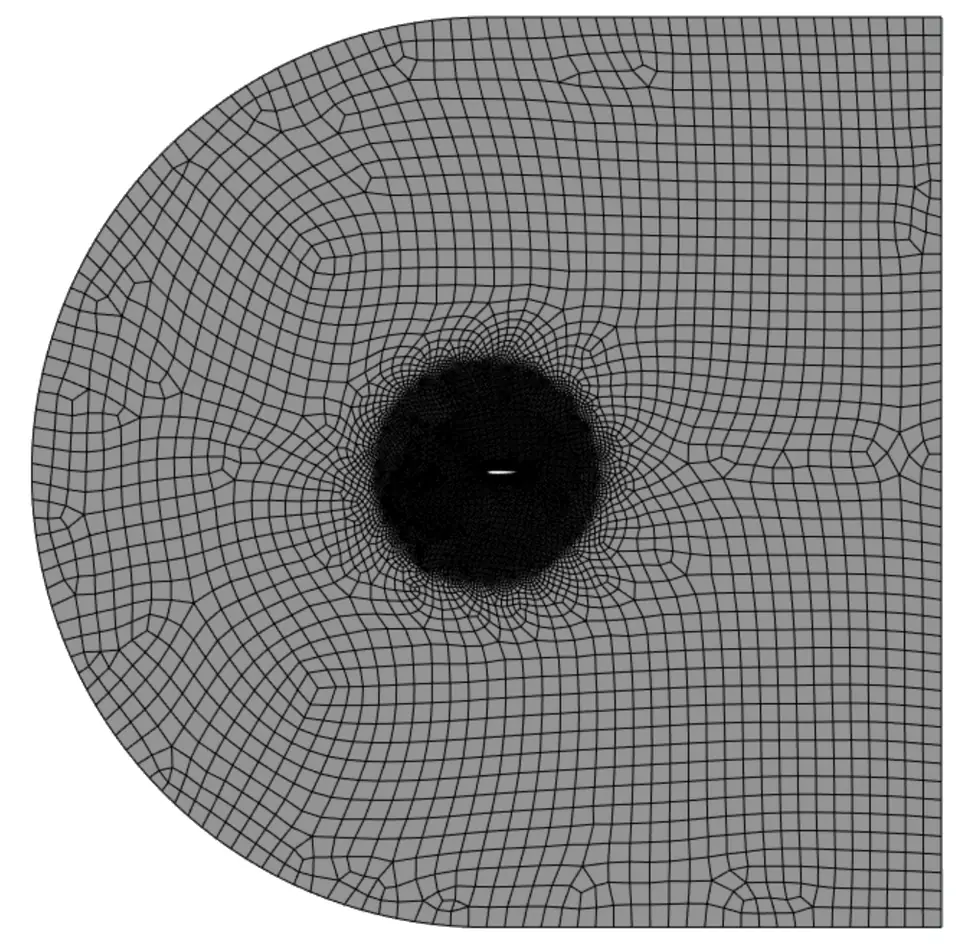
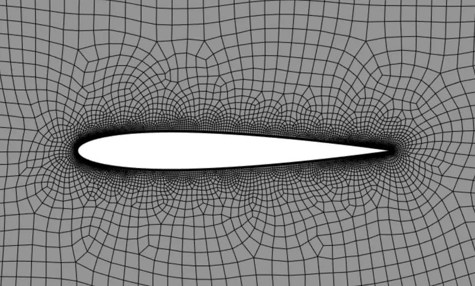
A layered meshing strategy resolves the boundary layer and near-body wake without paying for that resolution everywhere in a 12.5-chord domain: a coarse far field blended into a 3c sphere-of-influence refinement zone, 0.3% c edge sizing on the airfoil surface, and 10 inflation layers at a 1.2 growth rate.
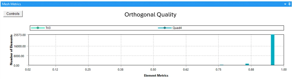
Orthogonal quality is above 0.9 for the large majority of elements, and the small number of lower-quality cells are concentrated exactly at the trailing edge, where the unstructured mesh becomes locally skewed.
- Cells
- 26,962
- Inflation layers
- 10, growth rate 1.2
- Surface cell size
- 0.3% of chord
- Refined zone
- 3 chords around the airfoil
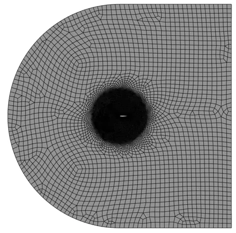
Coarse far field mesh blending into the finer sphere-of-influence refinement zone around the airfoil. 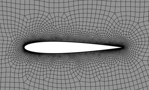
Close-up of the airfoil surface mesh and boundary-layer inflation layers. -
Solve the flow
ANSYS Fluent
The flow is modeled as steady, incompressible, and two dimensional, closed with the Realizable k-ε turbulence model and Standard Wall Functions. Discretization proceeds in two stages: an initial first-order-upwind solve for robustness, followed by a second-order-upwind solve for accuracy once the flow field is established, with all residuals converged to 10−6.
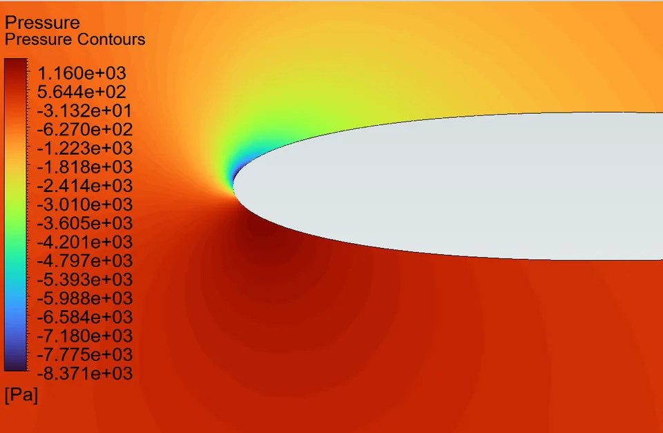
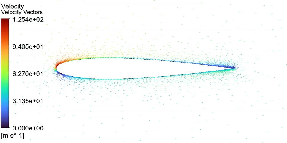
The pressure field shows the expected stagnation region just below the nose and a strong suction peak on the upper surface immediately downstream of it, and velocity vectors confirm the flow stays attached to both surfaces all the way to the trailing edge.
- Turbulence model
- Realizable k-ε
- Wall treatment
- Standard Wall Functions
- Discretization (final)
- Second-order upwind
- Residuals
- 10−6
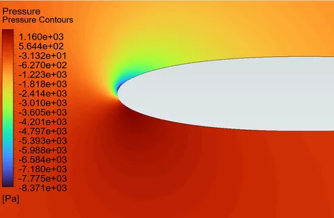
Pressure around the leading edge: stagnation region (red) and suction peak (blue). 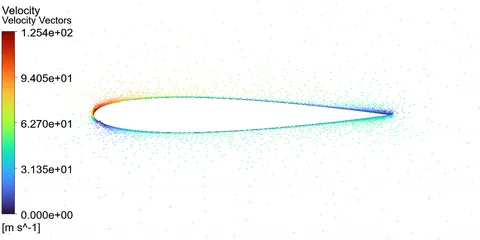
Velocity vectors confirm attached, forward-moving flow on both surfaces, with no separation. -
Compare with NASA data
CFD-Post
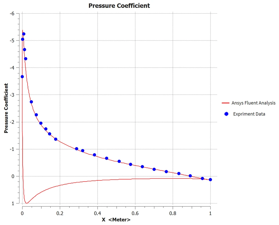
The computed pressure coefficient distribution was compared directly against published NASA wind tunnel measurements for this airfoil across the full chord, using a chordwise polyline built from the CFD-Post boundary-intersection tool.
The two curves overlap closely, including the sharp suction peak near the leading edge, which is the strongest evidence in this study that the overall lift-generating pressure field is being captured correctly, independent of how well the boundary layer itself is resolved.
- Lift coefficient
- 1.059 vs. ≈1.07–1.08
- Drag coefficient
- 0.0167 vs. ≈0.012
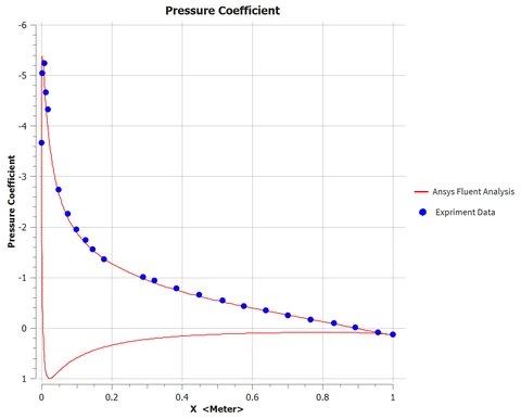
CFD pressure coefficient (line) against published NASA wind tunnel data (points), plotted with the conventional inverted vertical axis.
How I checked the results
Across the four validation and verification checks that matter most for this case, three are cleanly satisfied and the fourth points to one specific, fixable limitation.
3/4
validation & verification checks satisfied
The lift coefficient and surface pressure distribution match published NASA wind tunnel data to within a few percent, and the solution conserves mass to a relative imbalance far below any engineering concern. The drag coefficient over-predicts the experimental value by roughly 40%, an outcome that the y+ diagnosis below traces, most likely, to a specific, correctable meshing limitation rather than to a flaw in the turbulence model.
CFD result vs. published experimental value
Force coefficients shown as a percentage of the experimental reference value; 100% is an exact match.
| Validation / verification check | Computed result | Reference / target | Status |
|---|---|---|---|
| Surface pressure coefficient (Cp) | Close agreement across the full chord | Matches published NASA Cp distribution | Satisfied |
| Lift coefficient (CL) | 1.059 (≈1–2% low) | ≈ 1.07–1.08 (NASA reference) | Satisfied |
| Mass conservation | ≈4.8×10⁻⁷ kg/s against a ≈1490 kg/s through-flow | Net flux imbalance ≈ 0 | Satisfied |
| Drag coefficient (CD) | 0.0167 (≈40% high) | ≈ 0.012 (NASA reference) | Flagged, likely cause identified |
Near-wall resolution and y+ diagnosis
Because the pressure field is already shown to be accurate, the drag over-prediction has to come from somewhere else: the near-wall mesh. The non-dimensional wall distance y+ measures where the first mesh cell center falls relative to the layers of the turbulent boundary layer, and the Standard Wall Functions used in this study are only accurate when that first cell lands in the log layer, roughly 30 to 300.
Computed y+ spikes to roughly 90 right at the leading edge and dips to 3 to 5 just downstream of it, but sits at only 20 to 25 over most of the chord, below the required window. That places the first cell in the buffer region instead of the log layer, where the log law that Standard Wall Functions impose does not hold, so the computed wall shear stress loses accuracy; this lines up with the over-predicted drag coefficient carried through the whole solution.
y+ along the chord
Engineering judgment and recommendations
Beyond the pass-or-fail result, this study points to one dominant lever for improving it and a short list of items worth checking before extending the methodology to a new airfoil.
-
Flagged
Refine the near-wall mesh before trusting drag
The drag discrepancy most likely comes from a near-wall mesh that places the first cell in the buffer region rather than the log layer. Refining the boundary-layer inflation to y+ ≈ 1, or at minimum y+ ≈ 5 together with the Enhanced Wall Treatment, is expected to substantially improve the drag prediction without disturbing the already-accurate lift and pressure results.
-
Trailing-edge mesh quality needs local attention
A small number of skewed, poor-orthogonal-quality cells cluster at the trailing edge. They are a minor share of the total mesh, but sit exactly where the boundary layers from both surfaces meet, so they are worth resolving alongside the near-wall refinement above.
-
Mesh independence and far-field extent are still open
This study used a single mesh and a domain extent of 12.5 chord lengths. Neither has been formally shown to be independent of further refinement, so both remain on the list before the result should be treated as fully verified.
-
Confirm the methodology generalizes before reusing it
Before applying this meshing and turbulence-modeling approach to a new, less-characterized geometry, it is worth repeating this case with a second turbulence model (k-ω SST or Spalart-Allmaras) and at additional angles of attack, to check that today’s good agreement is not specific to this one operating point.
Technical details
Method, mesh and solver settings, and the flow-field analysis, for engineers who want to go deeper.
Method, mesh and solver setup Modeling assumptions, mesh controls, solver configuration and mesh quality
Method
The flow is treated as steady, incompressible, and fully turbulent, and solved with the Reynolds Averaged Navier Stokes equations rather than resolving every turbulent eddy directly.
Eddy-viscosity closure: τt = μt (∂ū/∂y), with μt supplied by the Realizable k-ε turbulence model
- All domain construction and surface meshing were done in ANSYS Meshing, starting from a single symmetric NACA 0012 profile.
- The flow is modeled as steady, incompressible, and two dimensional, closed with the Realizable k-ε turbulence model and Standard Wall Functions.
- Discretization proceeds in two stages: an initial first-order-upwind solve for robustness, followed by a second-order-upwind solve for accuracy once the flow field is established.
- Scope is limited to one operating point, one turbulence model, and one mesh topology; mesh-independence and multi-angle sweeps are identified as follow-on work, not performed here.
Mesh generation and solver setup
A layered meshing strategy resolves the boundary layer and near-body wake without paying for that resolution everywhere in a 12.5-chord domain.
| Region | Control | Setting |
|---|---|---|
| Far field | Background element size | Coarse, blended into the refinement zone |
| Airfoil vicinity | Sphere-of-influence radius / element size | 3.0 m (3c) / 5.0×10⁻² m (5% c) |
| Airfoil surface | Edge sizing / bias factor | 3.0×10⁻³ m (0.3% c) / 10.0 |
| Boundary layer | Inflation layers / growth rate / max. thickness | 10 / 1.2 / 6.0×10⁻³ m (0.6% c) |
| Mesh totals | Nodes / elements | 27,343 / 26,962 |
The solver was then configured to match the mathematical model above:
| Setting | Value |
|---|---|
| Solver type / time / space | Pressure-based / Steady / 2D planar |
| Turbulence model | Realizable k-ε, Standard Wall Functions |
| Fluid density / viscosity | 1.1767 kg/m³ / 1.009×10⁻⁵ kg/(m·s) |
| Discretization (final) | Pressure: 2nd order; Momentum, k, ε: 2nd order upwind |
| Convergence criterion (final) | 10−6, all residuals |
Mesh quality was checked on two standard metrics before moving to solver setup. Orthogonal quality is above 0.9 for the large majority of elements, and the small number of lower-quality cells are concentrated exactly at the trailing edge, where the unstructured mesh becomes locally skewed and is difficult to avoid without further local subdivision. This trailing-edge weakness is carried forward into the recommendations.
Flow-field analysis Velocity, pressure, streamlines and turbulence, compared with the behavior expected before solving
Each check below isolates one part of the converged flow field and compares it against the qualitative and quantitative behavior expected before the solver was ever run.
A1. Velocity Field & Boundary-Layer Development
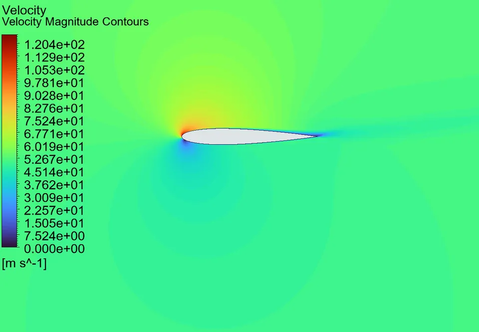
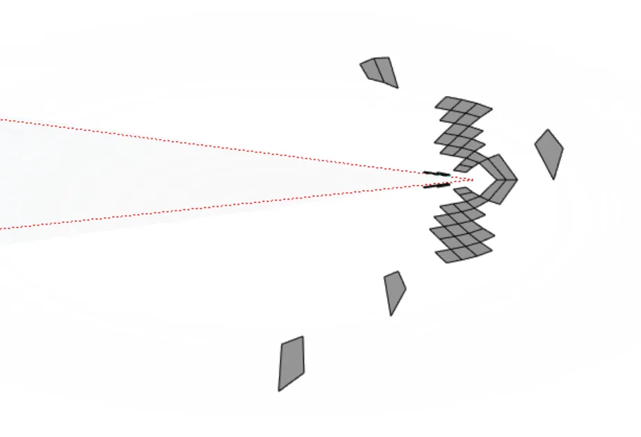
The velocity magnitude field accelerates around the nose and along the upper (suction) surface, exactly as expected for a positive angle of attack, and decelerates smoothly toward the trailing edge with no sign of large-scale separation.
Overlaying the mesh on the velocity field shows only a single control volume across the full boundary-layer thickness over much of the chord, a mesh-resolution issue that reappears quantitatively in the y+ check. Velocity vectors (step 3) confirm the flow stays attached to both surfaces all the way to the trailing edge, which rules out stall or separation as an explanation for the drag over-prediction.
A2. Pressure Field & Suction Peak
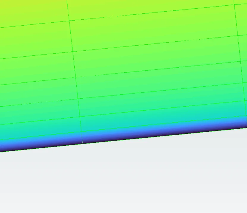
The pressure field shows the expected stagnation region just below the nose and a strong suction peak on the upper surface immediately downstream of it, where the flow accelerates most sharply around the leading-edge curvature.
Moving toward the trailing edge, pressure rises again, producing the adverse pressure gradient responsible for the boundary-layer thickening observed in A1. Because lift comes almost entirely from this pressure distribution rather than from viscous shear, an accurate pressure field is the main reason the lift coefficient comes out so close to the experimental value. The pressure field is shown in step 3.
A3. Flow Structure: Streamlines & Turbulence Production
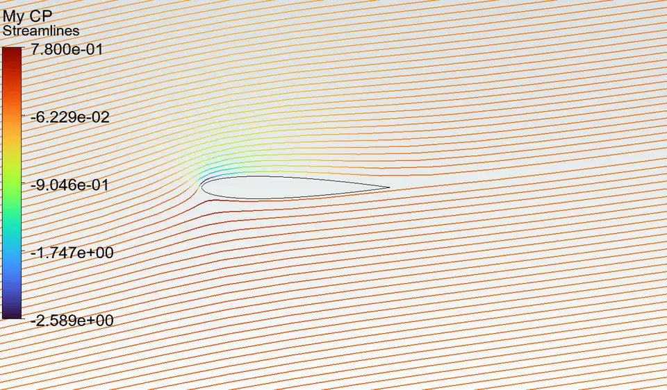
Streamlines seeded upstream of the airfoil and colored by pressure coefficient curve sharply around the suction peak before settling into a gentle wake, with no recirculation visible anywhere in the domain.
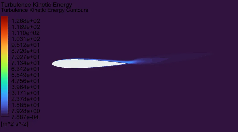
Turbulence kinetic energy is negligible in the free stream and concentrated almost entirely in the boundary layer and near wake, confirming that turbulence in this flow is generated locally by the airfoil rather than carried in from the inlet, so the estimated inlet turbulence values are not a significant source of uncertainty here.